Monkey Mind

Two simple approaches I like are the sum of distance-weighted contributions (SDC) and calculating the Mahalanobis distance from the training set.

Sum of distance-weighted contributions (SDC) is the easiest to calculate;

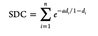
Where d_i is the distance between the ith molecule in the training set and the test molecule, a is adjustable parameter that modulates the distance penalty (typically 3) for molecule further away from the training set. Note that d is tanimoto distance, i.e. one minus tanimoto similarity.

def calc_sdc(ref_fps, query_fps):
    d = pariwise_distances(ref_fps, query_fps, metric="jaccard",n_job=-1, force_all_finite=True)
    sdc = np.sum(np.exp(-3*d/(1-d)),axis=0)

    return sdc

Fingerprints are ideally calculated by the same method as used to build the model.

Mahalanobis distance is definitely more difficult to say, and slightly trickier to calculate. It’s simply a measure of the distance between a point and a distribution . There are good implications for in python, Julia , etc. but something I thought would be useful to do would be to use the Facebook A.I. similarity search (FAISS) tool as it is super fast, easy to use, and so enabling application to large libraries.

def create_vector(vector):
    """
    Transform a vector to follow a unit Gaussian distribution using Mahalanobis transformation.
    """
    vector = np.ascontiguousarray(vector)
    xc = vector - vector.mean(0)
    cov = np.dot(xc.T, xc) / xc.shape[0]
    cov += 2 * np.eye(cov.shape[0])
    L = np.linalg.cholesky(cov)
    mahalanobis_transform = np.linalg.inv(L)
    return np.dot(vector, mahalanobis_transform.T)

With the vectors created from this function we create an in memory database of the transformed training vectors which we will then search.

def create_index(input_vector):
    """
    Create a FAISS index for a given set of vectors.
    """
    vector_dimension = input_vector.shape[1]
    index = faiss.IndexFlatL2(vector_dimension)
    index.add(input_vector)
    print(f"Index created with {index.ntotal} vectors")
    return index

Finally we search the indexed database and write the distances to file.

def main():
    if len(sys.argv) != 3:
        print("Usage: python AD_calc_mahalanobis.py <training_csv> <predict_csv>")
        sys.exit(1)

    training_df = pd.read_csv(sys.argv[1])
    predict_df = pd.read_csv(sys.argv[2])

    training_smiles = training_df["smiles"].tolist()
    predict_smiles = predict_df["smiles"].tolist()

    train_fps = smiles_to_fingerprint_array(training_smiles)
    predict_fps = smiles_to_fingerprint_array(predict_smiles)
    ###### SDC #############################################################


    sdc = calc_sdc(predict_fps, train_fps)

    predict_df["scd"] = sdc


    ######## mahalanobisDistance #################################

    array_train = create_vector(train_fps)
    array_predict = create_vector(predict_fps)


    index = create_index(array_train)
    distances, _ = index.search(array_predict, 1)

    predict_df["mahalanobisDistance"] = distances.flatten()

    ############# Write output ####################################
    predict_df.to_csv("test_cmps_with_distance.csv", index=False)
    print("Results saved to test_cmps_with_distance.csv")

if __name__ == "__main__":
    main()

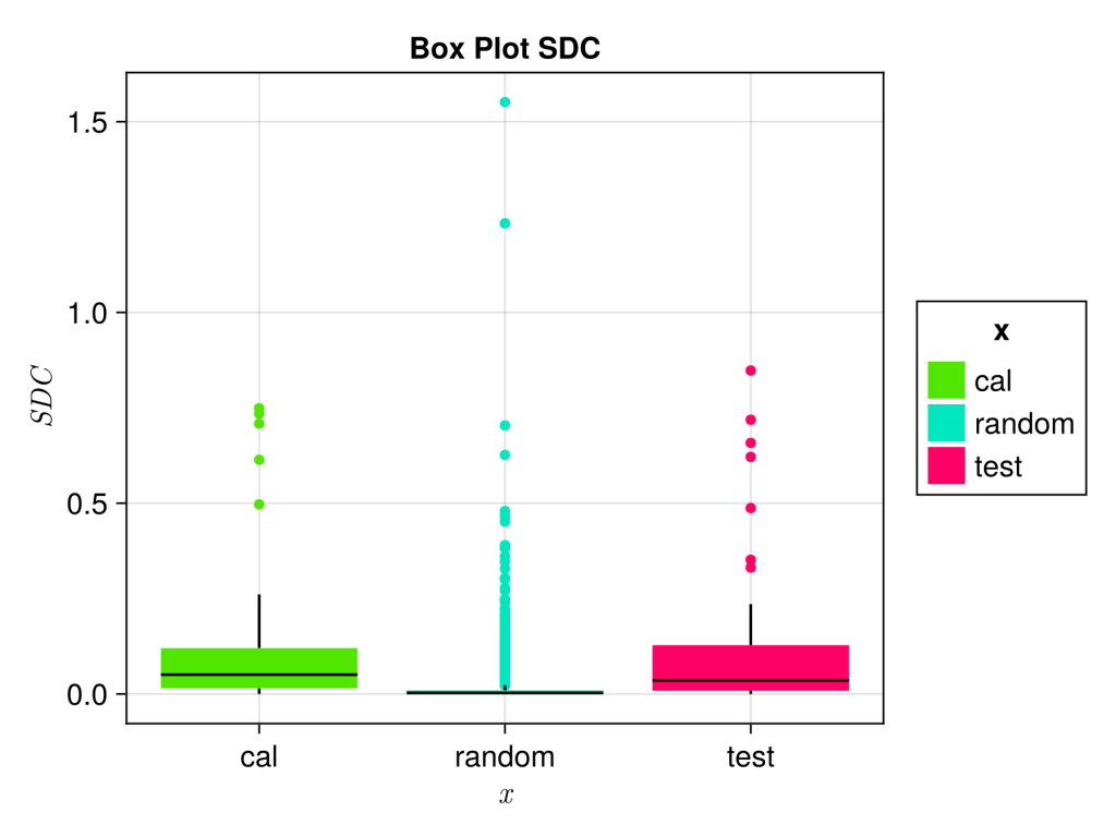
To sanity check everything we will plot the SDC of the external test set, calibration set and a 10000 random smiles generated using MoLeR sampling a chembl derived model provided. The box-plot was generate with AlgebraOfGraphics.

using Colors
using AlgebraOfGraphics, CairoMakie
using DataFrames, CSV

update_theme!(
           fontsize=16,
           markersize=8,
           Axis=(title=L"Box Plot SDC",))

# define colour scheme 
Sun_Orange_Bright = RGB(252/255, 229/255, 0)
Plant_Green_Bright = RGB(80/255, 230/255, 0)
Air_Blue_Bright = RGB(0, 230/255, 190/255)
Energy_Pink_Bright = RGB(255/255, 0, 100/255)

#read data
df_1 = CSV.read(ARGS[1], DataFrame)
df_2 = CSV.read(ARGS[2], DataFrame)
df_3 = CSV.read(ARGS[3], DataFrame)


y1 = df_1[!, :scd]
y2 = df_2[!, :scd]
y3 = df_3[!, :scd]

x = vcat(fill("test", length(y1)), fill("cal", length(y2)), fill("random", length(y3)))  # Group labels
y = vcat(y1, y2, y3)  # Combine columns into one vector

# Create a named tuple for AlgebraOfGraphics
df = (; x, y)
plt = data(df) * mapping(:x=>L"x", :y =>L"y", color=:x) * visual(BoxPlot) * data(df) * mapping(:x=>L"x", :y =>L"y", color=:x) * visual(BoxPlot)

colors = [Plant_Green_Bright, Air_Blue_Bright, Energy_Pink_Bright]

fg = draw(plt, scales(Color = (; palette = colors)))

save("BoxPlot.svg",fg, px_per_unit = 3)

As expected test set and calibration set look similar, whereas the random smiles looks more different.