As we know, pKa measurements are an important physical property, and much effort has been devoted to their calculation. I often feel that the devil is in the detail, which I think some QSPR models can gloss over, as such I was drawn to this paper by Gerald Monard group which uses atomic QM charges to predict the pKa of a range of simple acids with good accuracy (R2 = 0.955). The authors do a reasonable job exploring solvent models, DFT methods and charge models.
Detailed here are my attempts to reproduce their work with the tools I have available. Let’s break it down into the different parts: a) QM calculations b) extracting the charges c) Model evaluation
Code can be found at this GitHub
a) QM calculations
The Gaussian input file can be found in the papers supporting info, however for various reasons ORCA is by far my favoured quantum chemistry software package (and free for non-commercial use). As such I have translated the Gaussian .com file into a Orca .inp file.
--Link1--
%chk=CAS_62-23-7.chk
# opt nosymm freq M06L/6-311G(d,p) SCRF=(SMD,solvent=water) pop=nbo IOP(6/80=1)

CAS_62-23-7

-1   1
    C   -2.9342860000       -0.0000210000       -0.0000290000
    O   -3.4980180000       -1.1241640000        0.0014510000
    O   -3.4980380000        1.1241130000       -0.0013430000
    C   -1.4110770000       -0.0000090000       -0.0000170000
    C   -0.7017960000       -1.2046730000        0.0021260000
    C   -0.7018130000        1.2046660000       -0.0021430000
    C    0.6827570000       -1.2173540000        0.0021950000
    C    0.6827400000        1.2173660000       -0.0021760000
    C    1.3557730000        0.0000110000        0.0000190000
    H    1.2409380000        2.1448510000       -0.0037910000
    H   -1.2544120000        2.1372820000       -0.0037420000
    H   -1.2543830000       -2.1372960000        0.0037130000
    H    1.2409670000       -2.1448320000        0.0038240000
    N    2.8177720000        0.0000200000        0.0000390000
    O    3.4015070000        1.0813120000       -0.0012430000
    O    3.4015190000       -1.0812670000        0.0012640000
If you are well dosed with caffeine, you will have noticed that I have neglected the to include the “nbo” keyword in the transcription, while there is a simple interface with ORCA the NBO program, it requires a licence. The omission does compromise the predictive power, as the authors do get a better correlation with experimental results when the natural population analysis atomic charges are used rather than the Löwdin or Mulliken charges. As an alternative I will use the Minimal Basis Iterative Stockholder (MBIS) [Ayers2016] charges which weren’t looked in the paper.
!B3LYP D4 DEF2-SVP OPT FREQ MBIS
%PAL
NPROCS 12
END

%Method
WriteJSONPropertyfile True
End

%cpcm SMD TRUE
SMDSOLVENT "WATER"
end

* xyz -1   1
    C   -2.9342860000       -0.0000210000       -0.0000290000
    O   -3.4980180000       -1.1241640000        0.0014510000
    O   -3.4980380000        1.1241130000       -0.0013430000
    C   -1.4110770000       -0.0000090000       -0.0000170000
    C   -0.7017960000       -1.2046730000        0.0021260000
    C   -0.7018130000        1.2046660000       -0.0021430000
    C    0.6827570000       -1.2173540000        0.0021950000
    C    0.6827400000        1.2173660000       -0.0021760000
    C    1.3557730000        0.0000110000        0.0000190000
    H    1.2409380000        2.1448510000       -0.0037910000
    H   -1.2544120000        2.1372820000       -0.0037420000
    H   -1.2543830000       -2.1372960000        0.0037130000
    H    1.2409670000       -2.1448320000        0.0038240000
    N    2.8177720000        0.0000200000        0.0000390000
    O    3.4015070000        1.0813120000       -0.0012430000
    O    3.4015190000       -1.0812670000        0.0012640000
*
We run the calculations as normal, but given there are a few we just use a bash script to launch the calculations. Calculations are super speedy with ORCA6.0.1 and once we are done we have a xzy file and a property file in a json format (among many others).
for file in $(ls *.inp); do
   orca $file
done
b) Processing the output files
Things got a bit trickier here, I would be interested in hearing suggestions for a more elegant solution.
The first (Julia) script takes the outputted coordinate file (.xyz) and the property file (.json), uses the old & dependable obabel to write a mol2 file from the xyz, the script then update partial charges with those found in the ORCA json output. A key snippet is shown below.
function main(args)
    isempty(args) && error("Please provide a file name as an argument")
    file = args[1]
    base, _ = splitext(file)

    run(`obabel $base.xyz -omol2 -O $base.mol2`)
    atoms, bonds = read_mol2("$base.mol2")
    data = read_json("$base.property.json")
    new_charges = first.(data["Geometry_1"]["Mulliken_Population_Analysis"]["ATOMICCHARGES"])

    atoms_with_charges = add_charges(atoms, new_charges)
    output_file = "$base.mol2"
    write_mol2(output_file, atoms_with_charges, bonds)
end
The second script, grudgingly in python as I couldn’t workout an easy way of doing this in Julia, reads the newly modified mol2 file, locates the carboxylate with a SMARTS pattern and returns the partial charges for just the carboxylate group. Final we pivot the data and output a CSV file.
c) How did we do.
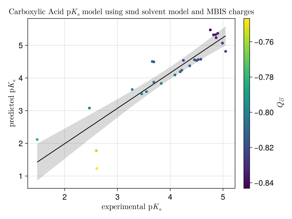
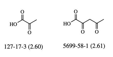
We did ok for quite a simple model, R2 = 0.81 compared to R2=0.955 from the authors, the coefficient of determination is brought down by a couple of outliers (acetopyruvic acid and pyruvic acid) where the proton can H-bond to the adjacent oxygen. Pleasingly MBIS charges worked pretty well, and maybe unsurprisingly better than Mulliken charges with all their known problems. Maybe NPA charges would work better. Thanks again to the authors Zeynep Pinar Haslak, Sabrina Zareb, Ilknur Dogan, Viktorya Aviyente and Gerald Monard.