Extracting uncertainty estimations from raw data.

I recently came across this blog article from Dr. Lewis Martin on Bayesian IC₅₀ fitting. The determination of uncertainty from raw data is something that is of interest to me. In the article Lewis use PyMC3, which is pretty popular, the analogues package in Julia is Turing so we will use that.

Imports

StaticArray.jl is mainly there to speed up the code, there maybe be better ways of doing this with threading or using a GPU.

using AlgebraOfGraphics, CairoMakie
using DataFrames
using  Turing, Distributions
using StaticArrays

Generate Fake Data

First define the concentration range for the x-axis.

# x points are in units of µM - they describe the 
# test ligand concentrations across a 9pt CRC
concs = [0.01, 0.032, 0.1, 0.32, 1, 3.2, 10, 32, 100]
# Convert concentrations to log10 Molar units
log_concs = -log10.(concs ./ 1e6)

Make up some pIC50 data for the y-axis using a sigmoid function.

function sigmoid(x; middle, slope, top, bottom)
    return top / (1 + ℯ^(-(x - middle) * slope) - bottom)
end

sigmoid_values = sigmoid.(log_concs; middle=6.1, slope=2, top=100, bottom=0)

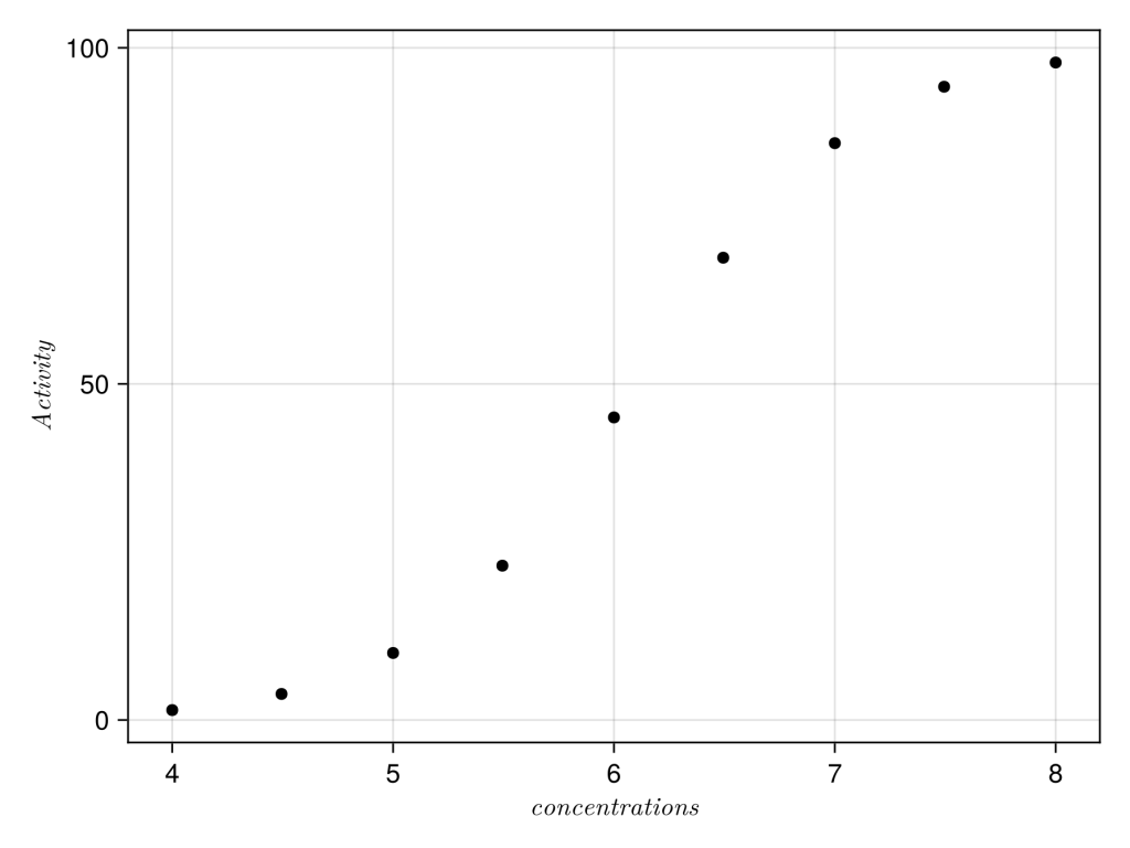
We’ll check the data by plotting the data, here we will use Algebra of Graphics

# plot initial data.
df = (; log_concs, sigmoid_values, )
xy = data(df) * mapping(:log_concs => L"concentrations", :sigmoid_values => L"Activity")
layers = visual(Scatter)
fg = draw(layers * xy)
save("figure1.png", fg, px_per_unit = 3)

Next we’ll re-plot the data with duplicates and noise.

#add some duplicates and noise.
concs = repeat(log_concs, inner=2)        
responses = repeat(sigmoid_values, inner=2)  
# Add random noise (Normal distribution with mean 0, std dev 5)
responses .+= randn(length(responses)) .* 5

With the data in hand we ready for modelling, first we define a model. Priors for top and bottom are inherently set to 100 and 0. For the variance we use the inverse gamma, the alternative would be the truncated normal err ~ Truncated(Normal(0, 20), 0, Inf). After this we build the model and then do a “No U–Turn Sampling” with 10,000 datapoints.

# Define the Turing model
@model function sigmoid_model(concs, responses)
    concs = SVector{length(concs)}(concs)
    responses = SVector{length(responses)}(responses)
    # Priors
    s² ~ InverseGamma(0.5, 20)
    midpoint ~ Normal(5, sqrt(s²))
    slope ~ Normal(0, sqrt(s²))
    bottom ~ Normal(0, sqrt(s²))
    top ~ Normal(100, sqrt(s²))
    
    # Sigmoid function: 
    proportion = @. top / (1 + exp(-(concs + midpoint) * slope)) - bottom
    # Likelihood (observed data with Gaussian noise)
    responses ~ MvNormal(proportion, s²)
end
end

model = sigmoid_model(concs, responses)
chain = sample(model, NUTS(), 10_000; tune=3000, target_accept=0.9)

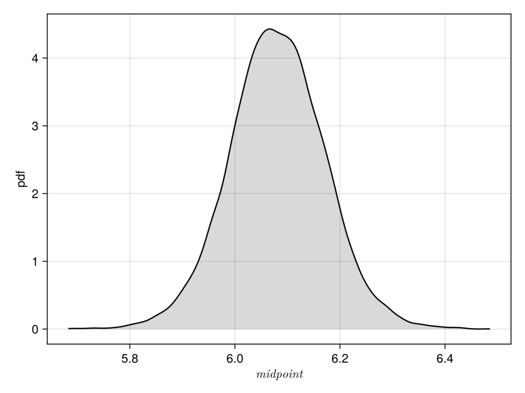
Finally plot the data as density plot, which looks good mean is approximately 6.1 and standard deviation is approximately 0.1.

df = DataFrame(chain)
df.midpoint = abs.(df.midpoint)
xy = data(df) * mapping(:midpoint => L"midpoint")
layers=AlgebraOfGraphics.density()
fg = draw(layers * xy)
save("figure3.png", fg, px_per_unit = 3)

Monkey Mind